Every machine learning system faces the same problem: what do you do when you have little data? A new customer signs up with 50 transactions. A new vendor appears for the first time. A new employee joins and needs to be routed invoices they have never seen before.

Traditional ML models fail here. They need hundreds or thousands of labeled examples per category before predictions become useful. In a multi-tenant SaaS application where each customer has their own data, this means every new account starts with zero accuracy and slowly climbs toward useful, if it ever gets there.

Aito takes a different approach. As a predictive database, it uses the structure of your data itself as prior knowledge. When a new entity appears, Aito does not start from zero. It starts from everything it already knows about entities like this one.

What is the cold-start problem?

The cold-start problem occurs when a prediction system encounters entities it has never seen in training data. A new vendor that has never appeared in your invoice history. A new employee who has never processed a document. A new product category with no purchase history.

Traditional approaches handle this poorly:

• Conventional ML (sklearn, XGBoost) treats each entity as an opaque label. If "Bob" never appeared in training, the model has no information about Bob. Accuracy for new entities typically drops below 50%.
• Rule-based systems fall back to default assignments. Every new vendor gets routed to the same person, creating bottlenecks.
• LLMs can generalize from descriptions and reason over retrieved examples, but carry per-call costs and latencies that make high-volume prediction uneconomical, as we show below.

A predictive database handles cold start differently because it understands the relationships between columns, not just the rows.

How Aito uses priors to solve cold start

Aito uses a layered system of Bayesian priors that operate at three levels. Each level addresses a different aspect of the inference problem, and they compose hierarchically to produce the final prediction.

Level 1: Property priors, the most powerful mechanism

This is where the real differentiation lies. When predicting a target field, Aito uses the properties of prediction candidates to infer about candidates it has never seen.

Consider predicting which employee should process a laptop purchase invoice. The system encounters Bob, a new IT manager with zero invoice history. Traditional ML would assign Bob a random probability. Aito does something different:

1. It knows Bob's department is IT.
2. It has observed that laptop invoices correlate with the IT department across all other processors.
3. Even with zero direct observations for Bob, the system infers that Bob is a likely processor for laptop invoices, because his properties match the pattern.

The prediction query is straightforward:

{
  "from": "invoices",
  "where": {
    "Description": "Laptop purchase",
    "Department": "IT"
  },
  "predict": "Processor"
}

Aito returns Bob with a meaningful confidence score, not because it has seen Bob process invoices, but because it understands what kind of person processes this kind of invoice. This is true zero-shot prediction.

Level 2: Analogy priors, structural pattern transfer

Analogy priors detect structural patterns across fields. When two fields share values in a systematic way (for example, the "to" field on an invoice and the "name" property of the processor), Aito discovers this pattern and uses it as prior knowledge.

If the system has observed that to:Alice often means processor.name:Alice, and to:Charlie often means processor.name:Charlie, it learns the general rule: the recipient name predicts the processor name. When it encounters to:Bob for the first time, the general pattern fires and provides signal, even though Bob specifically is new.

This is not simple string matching. The system quantifies the statistical strength of each analogy across all observed value pairs and weights its contribution accordingly.

Level 3: Distribution priors, adaptive baseline estimates

At the foundation, Aito uses adaptive priors on marginal probabilities. Instead of assuming every field value is equally likely (the naive approach), the system fits a Beta-Binomial distribution per field from the data:

• A field like category with 20 values gets priorP ≈ 0.05 (each value is roughly 5% likely before any evidence)
• A field like processor with 50 values gets priorP ≈ 0.02
• A field like id with thousands of values gets priorP ≈ 0.0001

These field-specific priors feed into every probability calculation. The system uses Hausser-Strimmer-style optimal shrinkage with variance-aware weighting to balance observed frequencies against prior beliefs. At small sample sizes priors dominate; as data accumulates, the data speaks for itself. Probability vectors are also structurally capped below 1.0 so the model cannot pin to a single candidate on thin evidence, which keeps calibration tight (the predicted confidence tracks the actual accuracy) across the long tail.

How the three levels compose

The prior levels are not independent alternatives. They compose hierarchically:

Distribution priors  →  set baseline probabilities per field
       ↓
Analogy priors       →  transfer structural patterns
       ↓
Property priors      →  use candidate attributes as evidence
       ↓
Final prediction with confidence score

Each level wraps the one below it. Distribution priors inform analogy priors. Analogy priors inform property priors. The final prediction incorporates evidence from all three levels, weighted by the statistical confidence at each stage.

This composition is why Aito handles cold start gracefully. A completely new entity benefits from all three levels simultaneously: baseline frequency estimates from distribution priors, structural pattern matches from analogy priors, and attribute-based inference from property priors.

What do the numbers look like?

We evaluated on a simulated invoice routing dataset: 100 companies, approximately 6,300 employees with globally unique IDs, and three prediction targets per invoice:

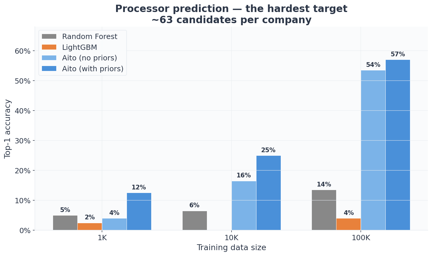
1. Processor: which employee should handle this invoice? (~63 candidates per company, the hardest target)
2. Acceptor: who should approve it? (~10 candidates per company)
3. GL Code: what accounting category? (32 codes globally)

Each invoice has a sender, product, and description text. Predictions for processor and acceptor are scoped to the valid employees of the invoice's company. The test set is 200 invoices, held out and never seen during training. We measure top-1 accuracy across three training scales: 1,000, 10,000, and 100,000 invoices. With n=200, individual numbers carry meaningful uncertainty (roughly ±5-7pp at the 95% level), but the directional patterns (which method scales, which one stalls) are consistent across targets and scales.

The data is synthetic, generated for scalability testing rather than realism. The text uses random syllable combinations instead of regular supplier names, and routing rules are probabilistic instead of deterministic. This makes the task harder for all methods than real invoice data would be. The absolute accuracy numbers would be higher on production data, but the relative comparison is fair because all methods face the same synthetic challenge.

We compared Aito against two well-engineered ML baselines: Random Forest (scikit-learn) and LightGBM, both using TF-IDF on text fields with company-scoped evaluation. LightGBM represents what an experienced ML engineer would build: it uses a local-index strategy that maps employee IDs to within-company indices, reducing the class space from 6,300 to ~247. This is a reasonable and common approach for multi-tenant classification, but as the results show, the encoding choice has dramatic consequences depending on the target. None of the prediction targets are used as input features for any method. The benchmark code, data, and methodology are available on GitHub.

The full picture

Processor (the hardest target, ~63 employees per company):

Training rows	RF	LightGBM	Aito (no priors)	Aito (with priors)
1,000	5.0%	2.5%	4.0%	11.0%
10,000	6.5%	0.0%	16.5%	26.0%
100,000	13.5%	4.0%	53.5%	52.5%

Acceptor (~10 candidates per company):

Training rows	RF	LightGBM	Aito (no priors)	Aito (with priors)
1,000	20.0%	32.5%	13.0%	25.0%
10,000	29.0%	48.0%	32.5%	41.0%
100,000	38.5%	76.0%	72.0%	70.0%

GL Code (32 codes globally):

Training rows	RF	LightGBM	Aito (no priors)	Aito (with priors)
1,000	34.0%	6.0%	57.0%	59.0%
10,000	60.0%	46.5%	68.0%	79.5%
100,000	53.5%	85.5%	65.5%	81.0%

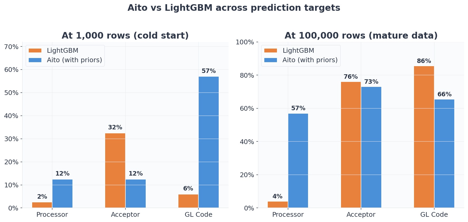
No single method wins everywhere. The story depends on the target.

Where Aito dominates: high-cardinality prediction with sparse data

Processor prediction is the hardest target: 63 candidates per company, sparse per-entity data, strong organizational structure. This is exactly the scenario priors are designed for.

At 1,000 rows (roughly 10 invoices per company), Aito with priors reaches 11%, more than 4x better than LightGBM (2.5%) and the only method meaningfully above random guessing (~1.6%). Both RF and LightGBM barely improve with more data: LightGBM actually drops to 0% at 10K and stays at 4% even at 100K. The local-index classification strategy that works for acceptor fails catastrophically for processor.

Why does LightGBM fail this badly? The encoding strategy that works for the smaller targets collapses the semantic space when there are many more candidates. Different strategies could avoid it, but that is precisely the point: getting the representation right for each target requires iteration and expertise, and you only discover the misfit after building and evaluating the pipeline.

By 100K, Aito reaches 52.5% while the best ML baseline (RF) manages 13.5%. The gap is roughly 4x. Aito without priors reaches 53.5%. Still dramatically better than both ML approaches.

Priors provide their largest lift at 1K, where they push processor accuracy from 4% to 11%, the difference between essentially random and the start of a useful signal. The gap narrows as data accumulates, and by 100K direct evidence dominates: the priors-on and priors-off scores converge within sampling noise. This is by design. Bayesian shrinkage lets the data speak for itself as the sample size grows.

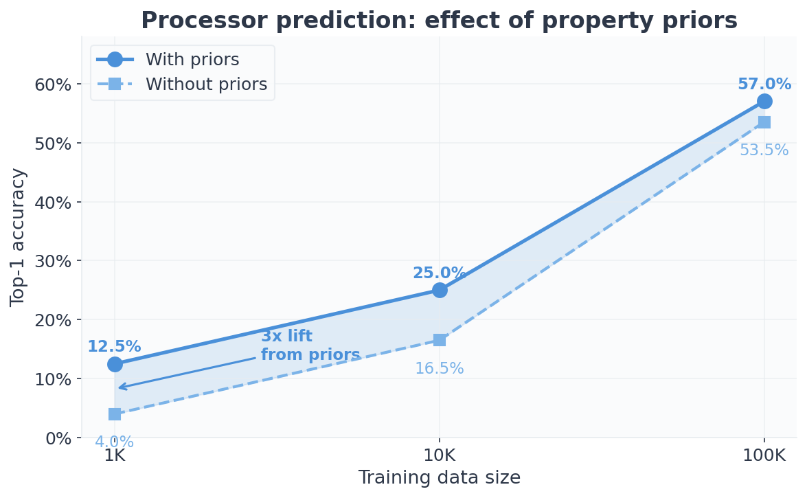
It is worth noting that even Aito without priors reaches 53.5% on processor at 100K, four times better than RF (13.5%) and thirteen times better than LightGBM (4%). Priors are not the only factor. Aito has a natural advantage with sparse data on both sides of the prediction.

On the input side, Aito forms models ad hoc at query time, using the full feature space. Every indexed column and every token within it is available as potential evidence, weighted by its observed co-occurrence with the target. A token that appeared once in training still contributes signal. A conventional ML pipeline commits to a fixed feature set at training time. If a column was not included in the TF-IDF matrix or the encoding scheme, it does not exist for the model.

On the prediction side, Aito does not need to enumerate all 6,300 employees as a flat class vector. It evaluates candidates through their properties and observed co-occurrences. An employee with zero direct observations still has a nonzero probability, through property priors but also through token-level co-occurrence with related entities. A conventional classifier assigns zero probability to unseen classes by definition. When both the input features and the prediction targets are sparse (exactly the situation in multi-tenant SaaS), these two advantages compound.

GL Code shows a similar pattern at small scales: Aito reaches 59% at 1K where LightGBM manages 6%. The GL code often appears in the invoice description text, and Aito's built-in tokenization picks up this pattern immediately without feature engineering.

Where LightGBM wins: low-cardinality targets at scale

LightGBM outperforms Aito on acceptor at every scale, and edges Aito on GL Code at 100K.

The acceptor field has only ~10 candidates per company. With fewer classes, gradient boosting can learn effective decision boundaries even without structural priors. LightGBM's local-index strategy (mapping employee IDs to within-company indices) works well here because the problem is small enough for a per-company decision surface.

At 100K, LightGBM reaches 76% on acceptor versus Aito's 70%. On GL Code at 100K, LightGBM reaches 85.5% versus Aito's 81.0%, a 4.5pp gap. With enough data and a manageable number of classes, gradient boosting is genuinely strong. The trade-off is that gradient boosting requires retraining whenever the data changes; Aito's predictions come straight from the database, with no separate training step to run.

Aito's GL Code trajectory is now monotone across scales (59% → 79.5% → 81%) where the earlier run had a slight dip at 100K. The growing description vocabulary that previously diluted token-level signals appears to be handled more cleanly by the new probability calibration. With a 200-sample test set, the cell-by-cell movements should be read with a ±7pp confidence band in mind, but the trajectory shape is the consistent story.

Notably, priors no longer make a measurable difference on GL Code at 100K once direct evidence is this strong, and they barely move acceptor. This is expected: GL code assignment is driven by invoice content, not organizational structure. Priors work best when the target has meaningful property-group structure. Department and role predict who processes an invoice, but they say less about which GL code to assign.

The overall score

Model	1K avg	10K avg	100K avg	Overall avg
Random Forest	19.7%	31.8%	35.2%	28.9%
LightGBM	13.7%	31.5%	55.2%	33.4%
Aito (no priors)	24.7%	39.0%	63.7%	42.4%
Aito (with priors)	31.7%	48.8%	67.8%	49.5%

Averaged across all targets and scales, Aito with priors achieves 49.5%: 48% higher than LightGBM and 71% higher than Random Forest. Aito wins 5 of 9 cells (all three processor cells, plus glCode at 1K and 10K). LightGBM wins 4 (all three acceptor cells, plus glCode at 100K, where the lead is now only 4.5pp).

The hidden cost: training time and maintenance

Accuracy is not the only dimension. LightGBM requires a separate model per prediction target. Training all three models takes:

Scale	RF (3 models)	LightGBM (3 models)	Aito
1K	~1s	~100s	0s
10K	~9s	~11 min	0s
100K	~100s	~40 min	0s

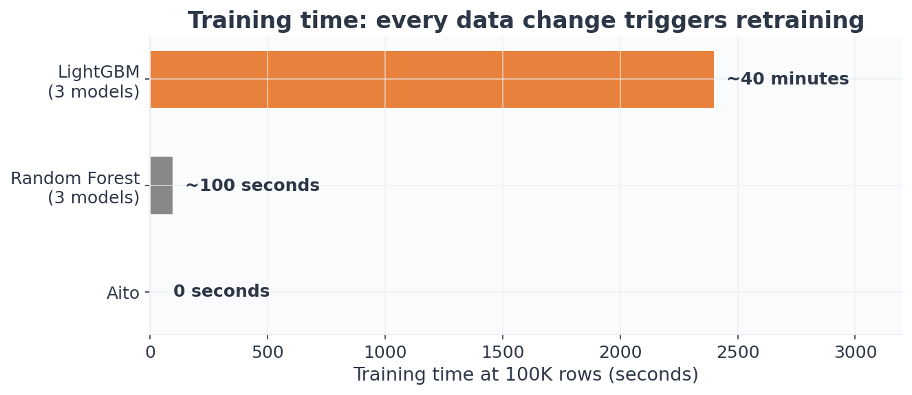
Forty minutes of training at 100K, and that repeats every time the data changes. New invoices, new employees, new GL codes: retrain everything. Aito predictions work immediately after data upload. For a SaaS product with 100 tenants, the operational difference between "retrain 3 models per customer on every data change" and "upload and query" is the difference between a data engineering pipeline and a database query.

What about using an LLM?

The obvious question in 2025: can you just throw an LLM at this? We tested GPT-5 mini with a TF-IDF retrieval-augmented setup. For each test invoice, the system retrieves the 15 most similar historical invoices by description similarity, includes the full employee list for the invoice's company (with names, roles, and departments), and asks the model to predict the processor.

This is a realistic RAG pipeline: the kind you would actually build if you were solving this with an LLM today. The model gets the same historical data and the employee properties directly in the prompt context.

Processor prediction, top-1 accuracy:

Training rows	Aito (with priors)	LightGBM	LLM + RAG
1,000	11.0%	2.5%	16.0%
10,000	26.0%	0.0%	16.0%
100,000	52.5%	4.0%	13.5%

At 1,000 rows, the LLM still leads: 16% vs Aito's 11%. This is worth pausing on. The LLM reads the employee list in the prompt, notices that an IT manager is a plausible processor for a laptop invoice, and reasons about the match. Through general intelligence, it is doing essentially what property priors do through statistical machinery: using candidate attributes to infer about unseen entities. The fact that both approaches sit in the same ballpark at small scale independently validates the insight that candidate properties carry real predictive signal.

But the LLM plateaus completely. From 1K to 10K, accuracy stays flat at 16%. At 100K, it actually drops to 13.5%. The RAG pipeline retrieves only 15 similar examples per prediction regardless of how much training data exists. More data in the training set does not help because the retrieval window stays fixed.

Aito scales in the opposite direction: 11% to 26% to 52.5%. The predictive database leverages the full distributional structure of the training data, not just a handful of retrieved examples. By 10K rows, Aito has overtaken the LLM. By 100K, the gap is roughly 4x.

The economics reinforce the point:

	Aito	LLM + RAG (GPT-5 mini)
Latency per prediction	19–45 ms	10–13 seconds
Throughput	20+ predictions/sec	~0.1 predictions/sec
Cost per 1,000 predictions	Flat rate	~$7
Cost per 100K predictions	Flat rate	~$700

The Aito latency numbers are measured per-target during this same benchmark run: GL code returns in roughly 20 ms across all scales, processor and acceptor in 35–45 ms. Latency is flat across scale: going from 1K to 100K training rows moves the per-query time by under 10 ms on every target. Each LLM call by contrast consumes roughly 4,500 tokens and takes 10–13 seconds. A batch of 10,000 invoices would take over 24 hours to process sequentially. A predictive database handles the same workload in minutes at a flat monthly rate, with response times comfortable behind a UI button.

When do priors matter, and when do they not?

The benchmark results make the answer concrete.

Priors provide the largest lift when:

1. The prediction target has meaningful properties that correlate with the prediction. Processor routing follows organizational structure: IT invoices go to IT people, management approvals go to managers. Department and role carry real signal. This is where priors shine, lifting processor accuracy from a random-noise floor to a useful starting signal at 1K rows.

2. Data is sparse. At 1,000 rows across 100 companies, there are roughly 10 invoices per company. Without priors, the system barely beats random guessing. With priors, it extracts structural patterns that compensate for limited direct observations.

3. The target has moderate-to-high cardinality. With ~63 processor candidates per company, there is not enough data per candidate for raw pattern matching. Priors fill the gap.

Priors provide little or no lift when:

• The prediction is driven by content, not organizational structure. GL code assignment depends on what the invoice describes (the GL code number often appears in the description text), not on who is involved. Adding basedOn=["role","department"] adds little to GL Code accuracy.
• The target has low cardinality. With only ~10 acceptor candidates per company, even basic approaches can learn the distribution. Priors help less than on processor, and LightGBM outperforms Aito on this target.
• Data is abundant. At 100K rows, the prior advantage narrows to within noise for processor and disappears for GL Code, where direct evidence is already strong. This is by design: the Bayesian shrinkage lets direct evidence dominate as the sample size grows.

What does this mean for your application?

If you are building a SaaS product that needs per-customer predictions, the cold-start problem is not a nuisance. It is a fundamental constraint on how fast your customers see value. Every day a new customer spends waiting for "enough data" is a day they question whether the integration was worth it.

A predictive database with layered priors changes the timeline. Predictions start working from the first rows of data. Accuracy improves as data accumulates, but it starts useful instead of starting useless.

One detail the accuracy numbers alone do not capture: Aito's predictions come with calibrated confidence scores. A prediction returned with 80% confidence is correct roughly 80% of the time. This means a workflow application can automate high-confidence predictions and route low-confidence ones for human review, extracting value even when top-1 accuracy is moderate. We cover calibration in depth in a separate post.

The query interface stays the same regardless of data volume. You do not need to configure priors, select features, or retrain models. Upload your data, query predictions, and the system handles the statistical machinery.

If you want to see how priors affect predictions on your own data, create a free Sandbox and upload a dataset. The effect is most visible when you compare predictions for established entities versus new ones with known properties.

Questions about how priors work in your specific use case? Reach us at hello@aito.ai.

Back to blog list