This post appeared first on Towards Data Science on July 8th, 2020.

Machine learning deals with probabilities, which means there’s always a chance for mistakes. This inherent uncertainty causes many decision makers feel uncomfortable with implementing machine learning and traps them in an endless chase for the magical 100% accuracy. The fear of mistakes nearly always pops up when I’m working with companies taking their first steps towards intelligent automation, and I get asked “What if the algorithm makes a wrong prediction?”

If this issue is not addressed, the company will very likely spend a hefty amount of resources and years of development time on machine learning without ever getting returns for their investment. In this article, I’ll show you the simple equation I use to relieve these concerns and get decision makers more comfortable with the uncertainty.

When is machine learning worth it

Just like with any investment, the feasibility of machine learning comes down to whether it generates more value than it costs. It’s a normal Return on Investment (ROI) calculation which, in the context of machine learning, weighs the generated value against the cost of mistakes and accuracy. So instead of asking “How do we get 100% accuracy?”, the right question is “How do we maximize ROI?”

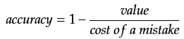
Determining the expected returns is quite straightforward. I usually begin opening up the business case for machine learning implementation by comparing its benefits against the potential costs in mathematical terms. This can be formalized in an equation which basically says “What’s left of the generated value after the cost of mistakes is accounted for?” Solving this simple equation allows us to estimate the profits for different scenarios.

Let’s look at the variables:

• returns: Generated net value or profit per prediction
• value: The new value generated by every prediction (e.g. assigning a document to the right category now takes 0.01 seconds instead of 5 minutes, so the value is 5 minutes saved)
• accuracy: The accuracy of predictions made by the algorithm
• cost of a mistake: The additional costs incurred by a wrong prediction (e.g. it takes 20 minutes for someone to correct the mistake in the system)

By flipping the equation around and setting returns to zero, we get the minimum accuracy required to generate net value. This is called break-even accuracy:

The equation gets more intuitive when plotted in a graph:

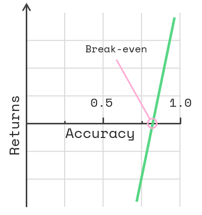
So let’s say each prediction saves you 5 minutes of work but it takes 20 minutes of extra work to fix a wrong prediction. We can now calculate the break-even accuracy to be 1–5/20 = 75%. Any improvement after this point brings concrete profits.

The above equation assumes us to blindly accept any prediction the algorithm makes and fix the errors afterwards. Sounds risky? We can do much better by extending the equation with confidence scores to lower the risks.

Optimizing ROI

A machine learning algorithm (done right) does not only spew out predictions, it also tells us how confident it is in every prediction. The majority of mistakes happen when the algorithm is unsure of its answer, allowing us to focus automation on the highest certainty predictions while manually reviewing the lowest few. Even though manual review does cost a bit of labor, it’s normally much cheaper than fixing a mistake later on.

Let’s choose a threshold which picks out 10% of the least confident predictions for manual review. The rest 90% will be handled automatically. This ratio is called confidence split. The accuracy in the high confidence bracket will now be considerably better since many of the mistakes are caught in the small unconfident bracket. This leads us to the extended equation. It says “What’s left of the generated value after the costs of mistakes and manual review are accounted for?”

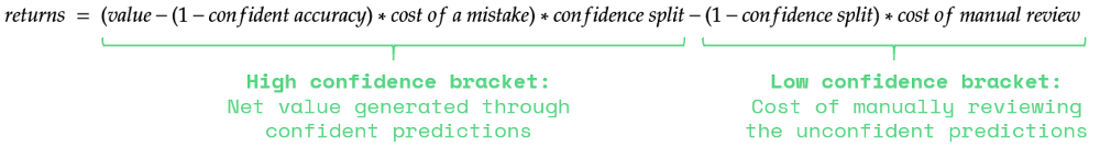
Let’s look at the variables:

• returns: Generated net value or profit per prediction
• value: The new value generated by every prediction
• confident accuracy: The accuracy of predictions in the high confidence bracket
• cost of a mistake: The additional costs incurred by a wrong prediction
• confidence split: The ratio of high confidence predictions (90% in our case)
• cost of manual review: The costs of manually reviewing the prediction

We can again flip the equation to calculate the break-even accuracy by setting returns to zero, like so:

We’ll solve it using the following variables:

• value = 5 minutes saved
• cost of a mistake = 20 minutes
• cost of manual review = 5 minutes
• confidence split = 0.9

Now the new break-even accuracy is 78%. Wait a minute, that’s higher than with the simpler equation, did it just get worse? Not quite! Remember that many of the mistakes are caught in the low confidence bracket, which significantly boosts the accuracy in the high confidence bracket. Even though the minimum accuracy requirement for break-even got higher, it is now much easier to achieve.

The ability to calculate the profitability of a machine learning algorithm in operation allows you to find the optimal accuracy. And no, it’s not 100%. As I discussed in my previous article, the development cost of any system increases exponentially while providing diminishing returns. With the above equations, you can estimate a realistic ROI and calculate the point where accuracy improvements incur more development costs than increase in returns in a time-frame of your choice. That’s the ROI-optimized accuracy.

Practical example

Let’s take a real world scenario and run through the whole thing. Imagine your Accounts Payable team handles 5000 invoices every month, and you’ve been presented the idea of automating a part of the process. More specifically, the proposed automation would categorize incoming invoices to match complex internal vendor codes, which is currently done manually. You need to figure out whether a machine learning approach is worth the effort to solve this task.

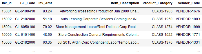
In terms of data, below is what you’ll be working with. You have a history of previously processed invoices and the correct “Vendor_Code” value for each. The task is to predict the right “Vendor_Code” for any new invoice. You can find the original dataset here.

To start off, use any machine learning library or tool you prefer and run a basic accuracy test for the data. I’m using aito.ai which gives me an accuracy of 78% after training with 4000 rows and testing with 1500 rows. If we use the same values and costs as before, we can calculate the monthly returns with the first equation:

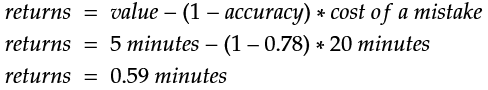
Using the simple approach which ignores the confidence scores, every prediction made by the algorithm with 78% accuracy saves you on average 0.59 minutes of work, or 35 seconds. That means almost 50 hours of work saved every month from processing 5000 invoices. Not bad.

Now let’s look at the equation which considers confidence scores. I compiled the results and confidence scores for each prediction into a neat table like below which allows us to divide them into high and low confidence brackets. In this case, any prediction with confidence lower than 0.21 will be reviewed manually. This threshold gives us the 90/10 confidence split.

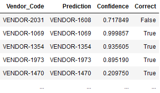
The accuracy in our high confidence bracket is an impressive 84%, and a measly 22% in the low confidence bracket. This makes the impact of utilizing confidence scores crystal clear. Now we can calculate the new returns when confidence and manual review costs are a part of the equation:

The extended approach nearly doubles the returns! Every prediction saves, on average, 1.15 minutes. Processing your 5000 monthly invoices now involves 95 hours less work even when the cost of mistakes and manually reviewing 10% of the predictions are accounted for. That’s pretty great!

Now you know the level of profitability you can currently achieve. And even better, you now have a tool to determine the feasibility of further machine learning development. For example, with the equation, you may calculate the returns for a hypothetical 90% accuracy and find the returns to be 183 hours saved monthly. Compare it to the estimated development costs of reaching the 90% accuracy and you’ll have factual data for deciding if further development is worth the investment.

Summing it up

As you’ve seen, machine learning should be approached just like any other investment. The inevitable mistakes are just a cost of doing business and they’re normal variables in our calculations. Armed with these equations, you know exactly when to start reaping the benefits of machine learning without playing a guessing game, and you can put the algorithms into production way earlier. Be freed from the endless grind towards 100% accuracy and start generating value already.

Done is better than perfect.

Back to blog list